A Beginner's Guide to Deep Learning (Part 2)

Disclaimer

If you haven't aren't familiar with Deep Learning concepts already, make sure to check out Part One Here, where I go over some essential concepts. I also make some disclaimers about me not being an expert! So with that being said, let's get started!

Prerequisites

I recommend being comfortable with the following concepts before continuing with this tutorial, although I'll try my best to spell everything out:

• python
• basic OS command line tools
• basic statistics concepts (validation, probabilities, etc)

Setup

I'm working in Ubuntu, so if you're working in Windows or Mac, and you want to follow these steps exactly, I recommend that you install an Ubuntu VM. Otherwise, if you want to stick with what you've got, you can use the next section as a loose guide as to what you'll need to get started.

Install Python 3 and pip

First, we need to install Python 3. We also need to install "pip" which is a package manager for python (something that installs other python modules). To do so, run

sudo apt install python3 python3-pip

Create a virtual python environment

Next, we need to create a "virtual python environment". We do this so that we can install python dependencies on a per-project basis, and not disturb any system-wide python packages. In other words, when you install or remove python packages, it does so at a local level, so you can add/remove packages without worrying about messing anything up.

To do so, run the following commands:

# Installs the venv module
sudo apt install python3-venv

# Creates a virtual environment called "dl-tutorial" in your home directory 
# in the folder ~/.venv
mkdir ~/.venv/dl-tutorial
python3 -m venv ~/.venv/dl-tutorial

Finally, if all went well run, the following command: source ~/.venv/dl-tutorial/bin/activate. If you did everything right, you should see (dl-tutorial) pre-fixed in your terminal. If you didn't, repeat these steps again, or look up guides for creating python virtual.

** Note that you will have to run source ~/.venv/dl-tutorial/bin/activate every time you start a new shell session!** This "activates" your virtual python environment.

Install Tensorflow, Keras, and All Dependencies

Now that you have your python environment set up, run the following commands. I recommend running them one by one to ensure you don't get errors along the way.

# Ensures that your virtual environment is activated
source ~/.venv/dl-tutorial/bin/activate

# Upgrades Setup Tools
pip install ––upgrade setuptools

# Installs tensorflow
pip install tensorflow

# Installs Keras
pip install keras

Tensorflow is a very-popular machine learning library developed and maintained by Google, and Keras is a wrapper around Tensorflow to make it a little friendlier to use. Unless your use-case is complex, or you are working on performance-critical code, you likely won't need to work with Tensorflow directly. That's why we'll be using Keras in this tutorial.

Solving our First Problem: Detecting Heart Disease

Sounds exciting, right? Well, to be clear, using neural networks for this particular example may not be the right tool for the job: traditional machine learning and statistical methods may be far simpler, and even more accurate, but for the sake of example, I think that this is an interesting use case. Also, this is not to be used in any real medical capacity. This is just for educational purposes!

Getting our data

Start by downloading the dataset here You will need to create an account, which kind of stinks, but I filled mine with totally fake information, so no need to worry about privacy.

The link above gives a pretty good description of the dataset, too: there are 14 columns in the dataset, and each row in the dataset contains information about a particular patient, such as their:

• Age
• Sex
• Chest Pain Severity
• Resting Heart Rate
• Max Heart Rate Observed
• Lots of Other Medical Metrics I don't understand :)
• Most importantly: a value of "1" if they have heart disease, and "0" if they don't.

I recommend opening up the file in Excel to understand how the data is represented.

Building the Neural Network

Alright, let's get started. First, create a file and call it dl_tutorial_01.py. Also, grab the heart.csv file and place it right next to the python file you just created (for simplicity).

Via Keras and Tensorflow, we'll be constructing a Feed-Forward Neural Network with a 13-node input layer, a 20-node hidden layer, ANOTHER 20-node hidden layer, and a single-node output layer.

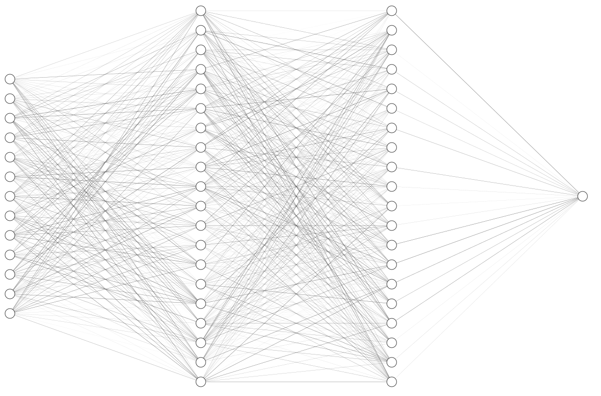A diagram of what our neural network will look like

Why are we building our network like this? Well, recall what our dataset looks like: we have 14 columns in our dataset: 13 of the columns tell us about the patient, while 1 of the columns tells us about the we want to know whether the patient has heart disease our not. Therefore, we have 13 "input variables", and one "output variable". Hence, 13 nodes in the input layer, and one node in the output layer.

In the statistics world, this is sometimes called a binary classification problem, meaning that we are simply searching for a YES or a NO answer to a certain question. Numerically (remmeber, neural networks only function with numbers), this can be represented simply with 1 or 0. So we want our network to output either a 0 or a 1, indicating whether the patient has heart disease or not.

Lets start with the following code, which loads the essential Keras imports, as well as the dataset itself.

import numpy
from numpy import loadtxt
from keras.models import Sequential
from keras.layers import Dense

dataset = loadtxt('heart.csv', delimiter=',', skiprows=1)

We're loading the data into an array of arrays. To see what that looks like, let's print one row. Add the following line:

print("Here is the first row of the heart.csv dataset:")
print(dataset[0])

To run what we have so far, run the following command: python dl_tutorial_01.py. You should see something like this (aside from an error about not being able to load a dynamic library, which you can ignore for now):

Here is the first row of the heart.csv dataset:
[ 63.  1.  3.  145.  233.  1.  0.  150.  0.  2.3   0.  0.  1.  1. ]

This should match the first row in the dataset. Next, we want to separate the 13 input variables (age, sex, heart rate, etc), and single output variable (1/0 for "do they have heart disease"). We can do this using the code below:

x = dataset[:,0:13]
y = dataset[:,13]

Now that we have our dataset, it's time to build our Neural Network as described above

model = Sequential()
model.add(Dense(20, input_dim=13, activation='relu'))
model.add(Dense(20, activation='relu'))
model.add(Dense(1, activation='sigmoid'))
model.compile(loss='binary_crossentropy', optimizer='adam', metrics=['accuracy'])

Let's break this down. The model.add() statements add layers to the model. The first statement specifies the input dimension, which is 13 nodes (corresponding to how many input variables in our dataset). They also specify something called an "activation function".

Something I've glossed over until now is that nodes don't simply take in values, sum them all up, and pass that sum along: it instead performs some kind of function on the sum before passing it along to the nodes in the next layer. The particular function being performed on it is the "ReLU" function, which is described here. There are multiple functions to choose from, but for hidden layers, ReLU is the general, accepted choice.

You'll notice that, for the final layer, we have a one-node layer, with a different activation function: a sigmoid function.

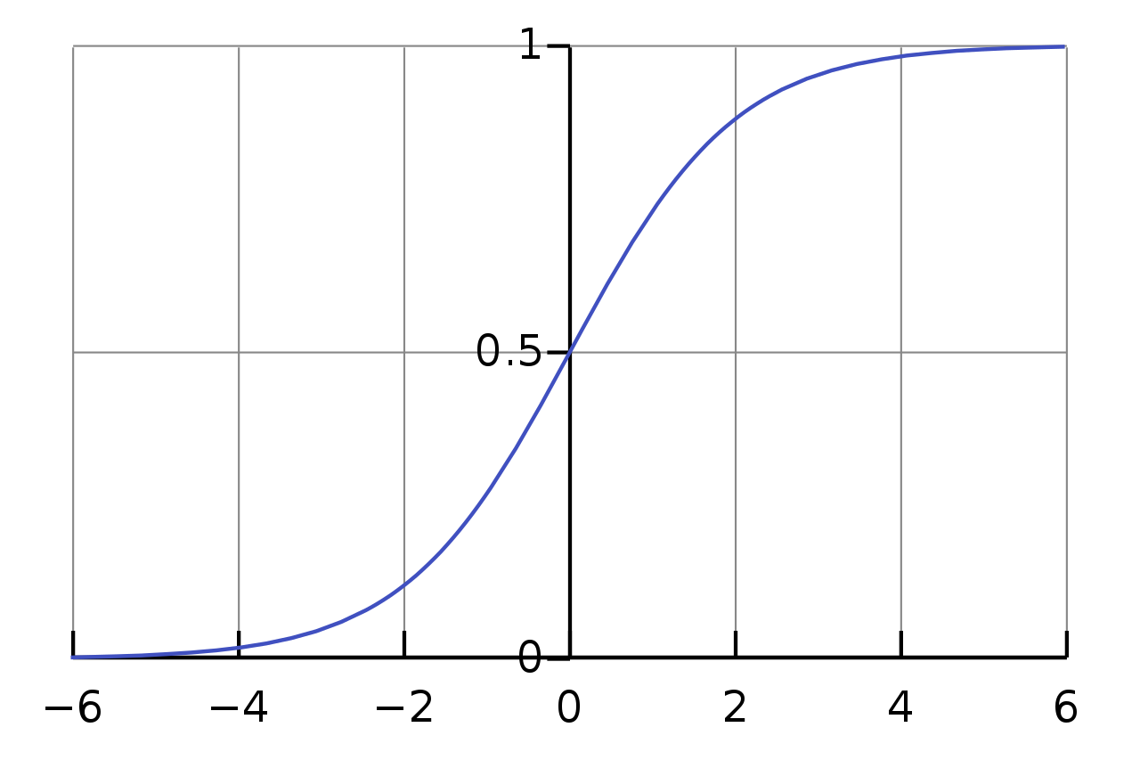A Sigmoid function, identified by it's distinct "S" shape

This function constraints the output from 0 to 1, which is exactly what we need for our binary classification task.

Finally, the model.compile() statement builds the model. Take note of the loss='binary_crossentropy' parameter: the loss function is used to evaluate how "correct", numerically, your neural network's prediction is when compared to the actual correct answer. You might think, "just take the absolute difference between the two numbers", but it's far more complicated than that. Loss functions aren't exclusive to Deep Learaning, and there are specialized functions for specific use cases. In our case, we use "Binary Cross Entropy", which, as explained in this great post, is best suited for binary classification problems.

Also note the optimizer='adam'. This specifies the gradient descent algorithm that we're using, something that I handwaved in Part 1. For the purposes of this post, you simply need to understand that the Adam algorithm is the most popular choice for Gradient Descent in Neural Networks, which is used to help the model now how to slowly adjust its edge-weights towards the "correct" set of edge-weights.

Training the model

Now that we've built the model and specified how it should be trained, we can actually train the model by adding the code below:

model.fit(x, y, epochs=150, batch_size=10)

This should take around 10 seconds or so, depending upon the speed of our CPU. This command is saying to go through the entire dataset 150 times, using batches of 10 samples to train the network.

Once it's done, congrats! We now have a (fake, toy) heart disease detector in python! Let's try it out on the first patient in the dataset, which we KNOW has "1" in the last column, indicating that they do. Add the following code and run it.

prediction = model.predict(x[0:1])
print("Prediction: "+str(prediction[0][0]))
print("Ground Truth: "+str(y[0]))

Which will produce output something like this (your numbers may vary, due to the fact that that many factors in these algorithms are initialized to random numbers):

Prediction: 0.9282936
Ground Truth: 1.0

You should see output concluding that our model is pretty confident that the first patient has heart disease. So what about for the entire dataset as a whole? It would be far too time consuming to manually check out model's output against the every value in the dataset, so we'll automate this process in the next section.

Evaluating the model

To evaluate our model, we'll use one commonly-used metric, "accuracy", which simply compares how many times our model guesses the correct answer relative to the total number of guesses. This is a one-liner in Keras, but for your own understanding, this logic is illustrated in the pseudo-code below

correct = 0
for (sample in samples):
  x = [sample][0]
  y = [sample][1]

  # if the model is 50% confident or more, consider it's output 1, otherwise consider its output 0
  prediction = round(model.predict(x)) 

  # If the model's output matches the label, then consider its prediction correct
  if (prediction == y)
    correct += 1
  
accuracy = correct / len(samples)

Here's how easy Keras makes it:

_, accuracy = model.evaluate(x, y)
print('Accuracy: %.2f' % (accuracy*100))

Your should see an accuracy value somewhere around 80%.

Recap

If you've gotten this far, then you should have working code at this point! Here's the final copy of the code:

# Here, we're using Keras and Tensorflow to use feed-forward neural networks to predict heart disease, 
# using the heart_disease.csv dataset.

# Import feedfoward keras stuff
import numpy
from numpy import loadtxt
from keras.models import Sequential
from keras.layers import Dense

# Load the dataset, and
dataset = loadtxt('heart_disease.csv', delimiter=',', skiprows=1)
x = dataset[:,0:13]
y = dataset[:,13]

# Build the Neural network. 2 Hidden layers.
model = Sequential()
model.add(Dense(20, input_dim=13, activation='relu'))
model.add(Dense(20, activation='relu'))
model.add(Dense(1, activation='sigmoid'))
model.compile(loss='binary_crossentropy', optimizer='adam', metrics=['accuracy'])
model.fit(x, y, verbose=0, epochs=150, batch_size=10)

# Do a single prediction, just for fun
prediction = model.predict(x[0:1])
print("Prediction: "+str(prediction[0][0]))
print("Ground Truth: "+str(y[0]))

# Asses the accuracy of the model.
_, accuracy = model.evaluate(x, y)
print('Accuracy: %.2f' % (accuracy*100))

Summary

At this point, you've installed Tensorflow, Keras, built and trained a Neural Network on a binary classification task, and achieved around 80% accuracy. There are many more directions you could take your research from here. I've glossed over many things, such as:

• The math behind backpropagation and gradient descent
• Loss functions
• How to evaluate the correctness of your Neural Network (accuracy is simply one metric)
• Improving the accuracy of your model
• Using other metrics (other than accuracy) to evaluate your model
• Training Vs Testing your model (we "evaluated" our model on data it's already seen before, which is really not what you should be doing. We only did so for simplicity).

Hopefully I've given you enough to pique your interest in furthering your own research. As you can see, there's quite a bit of overlap between Deep Learning, machine learning, computer science, math, and statistics, so don't despair if it all seems a little overwhelming!

Stay tuned for another post, where I'll tackle another more-complicated task using Keras and machine learning!